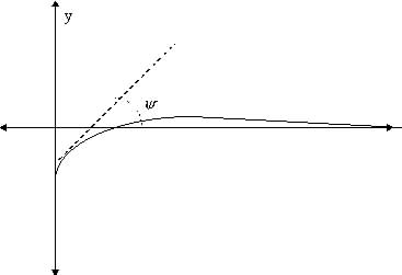
We now attempt to apply equation (29) to the model the development of a grain boundary groove at the point of contact of two crystals. The system is assumed to be symmetric and the surface initially flat. The gradient of the slope at the root of the groove is considered fixed (Mullins 1963). Far from the groove the surfaces will remain flat with constant surface gradients. Continuity is assumed at the root of the groove. The system is pictured below.
The boundary conditions for the symmetric groove are
fixed slope:
![]() (constant) (30)
(constant) (30)
Grain boundary neither absorbs nor emits material:
![]() (31)
(31)
Surface is flat far from the grain boundary (up to as many derivatives as required):
![]() (32)
(32)
Initially the surface is flat:
![]() (33)
(33)
Under the similarity reduction (13) the boundary conditions transform to
![]() (34)
(34)
![]() (35)
(35)
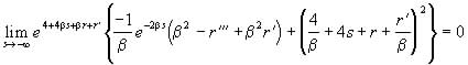
![]() (36)
(36)
When we apply the symmetry invariants (26) and (27) to these the boundary conditions become:
![]() (37)
(37)
 (38)
(38)
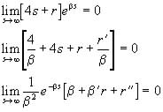 (39)
(39)
Unfortunately, while the evolution equation (25) was reduced by the symmetry transformations such uncoupling was not possible for the boundary conditions. The complicated nature of the transformed boundary conditions mean that it is unlikely that the transformed evolution equation (29) is any easier to use than in its original form.