To gain a better understanding of the principles behind chaos and strange attractors it is useful to look at a simpler system that Lorentz’s convection model. An ideal example is the driven non-linear pendulum. This has the dimensionless equation of motion:
![]()
Here ![]() is the angular position in radians, q is the damping parameter, g is the amplitude of the driving force, while
is the angular position in radians, q is the damping parameter, g is the amplitude of the driving force, while ![]() is the frequency of that force.
is the frequency of that force.
It is common to use the small angle approximation for this equation with ![]() . This allows the equation to be integrated, but means that the pendulum will either undergo regular motion or, without a driving term, eventually stop swinging altogether. For the type of motion that we desire to study, this approximation is invalid and hence the equation can no longer be solved analytically.
. This allows the equation to be integrated, but means that the pendulum will either undergo regular motion or, without a driving term, eventually stop swinging altogether. For the type of motion that we desire to study, this approximation is invalid and hence the equation can no longer be solved analytically.
It is useful to rewrite the second order differential equation of the pendulum’s motion as a system of first order differential equations:
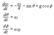
This time independent system of equations is said to be in autonomous form. The ![]() variable is the phase of the driver.
variable is the phase of the driver.
Phase Portraits
(I will be adding Java applets in the near future to display the phase portraits mentioned below)
The dynamical variables of the system, in this case the angular position ![]() and velocity
and velocity ![]() , are the coordinates defining the system’s phase space. In the two dimensional case, the variables can be plotted to display a phase portrait of the dynamical behaviour. By varying the parameters of the equation for the non-linear pendulum and then plotting the resulting phase portrait a wide range of behaviour can be observed.
, are the coordinates defining the system’s phase space. In the two dimensional case, the variables can be plotted to display a phase portrait of the dynamical behaviour. By varying the parameters of the equation for the non-linear pendulum and then plotting the resulting phase portrait a wide range of behaviour can be observed.
We start by setting the driver strength, g, to 0, the damping parameter q to 2.0 and ![]() to (4,-3). The phase portait shows the points spiralling in to (0,0) which, in the pendulum’s case, corresponds with the pendulum motionless and vertical, with the weight below the pivot. The phase portrait is then redrawn with a different starting point at (-3,0). The points again spiral in, this time from the opposite direction. In fact, if we take any point, with one exception, the trajectory of the phase points will eventually end at (0,0). If the physics of the situation are considered then this makes perfect sense. The damping term means that the pendulum is losing energy (this would be through friction in a real system) and as such the swing is decreasing until the pendulum comes to rest. In other words, with a non-zero damping parameter and no driving force to replace the energy lose, the pendulum is a dissipative system.
to (4,-3). The phase portait shows the points spiralling in to (0,0) which, in the pendulum’s case, corresponds with the pendulum motionless and vertical, with the weight below the pivot. The phase portrait is then redrawn with a different starting point at (-3,0). The points again spiral in, this time from the opposite direction. In fact, if we take any point, with one exception, the trajectory of the phase points will eventually end at (0,0). If the physics of the situation are considered then this makes perfect sense. The damping term means that the pendulum is losing energy (this would be through friction in a real system) and as such the swing is decreasing until the pendulum comes to rest. In other words, with a non-zero damping parameter and no driving force to replace the energy lose, the pendulum is a dissipative system.
The point (0,0) is called an attractor. By approximating the non-linear equations with linear forms and assuming that their behaviour will not differ substantially around critical points it can be shown (see Derrick and Grossman, 1987) that the damped pendulum with initial conditions ![]() and
and ![]() will spiral in towards the point
will spiral in towards the point ![]() closest to it, where n is an integer. A useful analogy is to think of a series of bowls (imagine, somehow, that there are no gaps between them) with the points of
closest to it, where n is an integer. A useful analogy is to think of a series of bowls (imagine, somehow, that there are no gaps between them) with the points of ![]() at the centres. These are equilibrium points where the potential energy is lowest. The peaks of the walls separating these “bowls” or basins of attraction are at
at the centres. These are equilibrium points where the potential energy is lowest. The peaks of the walls separating these “bowls” or basins of attraction are at ![]() and are unstable critical points called saddle points. At these points the pendulum would be pointing vertically upwards. The merest push will send it back down again.
and are unstable critical points called saddle points. At these points the pendulum would be pointing vertically upwards. The merest push will send it back down again.
Suppose we now use a non-zero driving force. We start off with a value for g that’s not too strong, the intention is just to overcome the energy loss due to damping. If we plot the phase diagram we see that the attractor is no longer a single point at (0,0) but now a closed, almost elliptical, curve. The pendulum is swinging back and forth tracing out the same path, undergoing regular motion.
If we increase the driving force a bit more, we now find that instead of just tracing out one loop, the pendulum must now swing through two loops until it reaches the same point again on the phase diagram. The pendulum’s period has doubled. Tweak g a bit higher and the period doubles once more and four loops appear. This doubling continues as g is increased until a point is reached where, in order to return to the same point, the pendulum must pass through an infinite number of swings. In other words, the motion of the pendulum ceases to be regular and becomes chaotic.
The question may be asked, “How do we know from the phase diagram that the pendulum isn’t just going through a lot of swings instead of an infinite number?”. After all, as the number of periods increases, it becomes pretty difficult to trace a path along the points on the phase diagram. A solution to this problem is to use a Poincare section. This is done by taking “snapshots” of the phase space at time intervals equal to ![]() , where n is an integer and
, where n is an integer and ![]() is just a phase term.
is just a phase term.
Using the Poincare section we find that regular motion with a single period means that only one point is plotted. A period doubling adds another point, and each extra period doubling adds two more points. It is when a chaotic state is reached that the Poincare section looks really interesting. Instead of points, long “wavy” lines are now seen. If we were to magnify a section of these lines we would see that they were actually composed of bunches of lines. If we magnified one of these lines we would see that this was also composed of another bunch of lines. In fact we could continue the magnification indefinitely and we would still see much the same thing. Hence, the pendulum’s attractor is now a fractal, just like the attractor for Lorentz’s equations.
Unfortunately, this detail isn’t really available from the sections plotted here due to the high number of iterations required. The graphics really provide just a general impression of the shape. For better graphics take a look at the plots in Baker and Gollub.
It should be noted that the driven pendulum is no longer a dissipative system, as the driving force “replenishes” the energy lost by the damping. What this means is that areas (and volumes) of phase space are conserved with time. In a dissipative system, they decrease. The Lorentz system is dissipative, but because of its strange attractor it does not dissipate to zero.
If we were to plot a diagram of the values of the angular velocity, w, against an axis of increase g we would notice some very interesting results. This will have to be imagined because my C++ programming skills are not up to writing graphics routines yet and good old uncompiled BASIC will take a very long time to do one of these diagrams for a pendulum. For a while we would see only a single line. This represents single period regular motion. At a certain point the line splits in two (the correct term is bifurcates and these plots are called bifurcation diagrams), which is where a period doubling occurs. Further on it bifurcates again, then again, until a chaotic state is reached, appearing as a “fuzz” of points.
Moving through the chaotic regions we find windows of odd periodicity, such as period 3 appear. By Sarkovskii in 1964 and Yorke and Li in 1975 we know that if a system has an odd period, then it is capable of a chaotic state.
If we continue to increase g a point is reached where period two motion returns. Again bifurcations will reoccur for values of g somewhere above this and chaos will eventually appear again. It is interesting to compare the differences between the Poincare sections of the chaotic regions after these even period sections. It is as if the original points have been pulled out and folded. Indeed, this is a rough way of describing a series of transformations. It is this aspect of fractals which forms the second part of this discussion.